 NexGPU-算力租赁,GPU服务器,GPU云算力,AI服务器租用-新闻博客
Uneven expert load in MoE manifests in two stages with different symptoms and root causes. Before diving into debugging, determine which scenario you are in:
- During training or fine-tuning: The routing itself is degrading. A few "hot experts" take most of the tokens, while others receive almost no input and become "dead experts." If a capacity limit (capacity factor) is set, the token drop rate also increases. The root cause is usually in the router and the balancing loss.
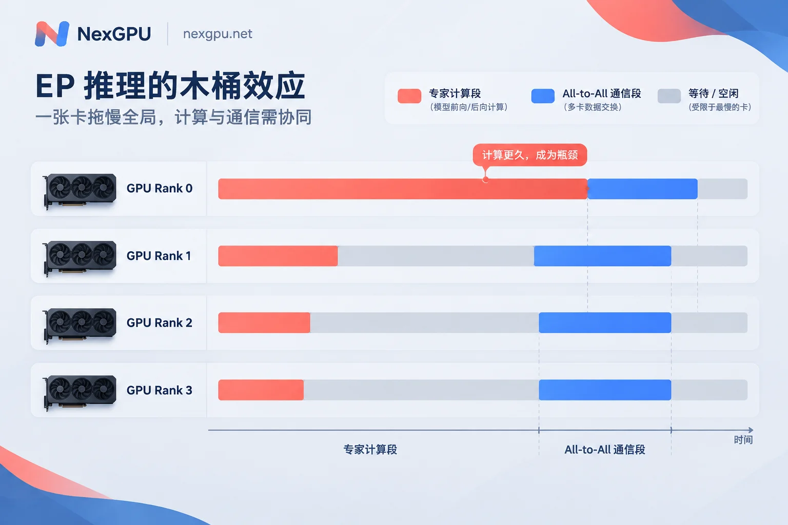
- During multi-GPU inference with expert parallelism (EP) enabled: Model weights are fixed, and the problem manifests as different computation times across GPUs. Faster GPUs must wait for slower ones at All-to-All communication points, significantly increasing tail latency of TTFT and TPOT. The root cause is often in the request data distribution and how experts are placed across GPUs.
If you are doing inference but using tensor parallelism instead of EP, each expert's weights are split across all GPUs, and uneven expert popularity generally does not cause GPUs to wait for each other. In this case, if throughput is not improving, first check the parallelism strategy and interconnect following the ideas in Why Multi-GPU Inference Throughput Doesn't Double.
Training or Fine-tuning: Check Routing in Four Steps
Step 1: Count tokens assigned to each expert layer by layer
This step requires two sets of numbers: the actual token proportion f_i for each expert, and the average probability p_i assigned by the router. Plot histograms or heatmaps per layer to check for extreme skew. A single-GPU small-batch forward pass can accomplish this. For example, with Mixtral in Hugging Face Transformers:
import torch

@torch.no_grad()
def expert_load(model, batch, top_k=2):
    out = model(**batch, output_router_logits=True)
    mask = batch["attention_mask"].flatten().bool()  # 去掉 padding token
    report = []
    for layer, logits in enumerate(out.router_logits):
        logits = logits[mask]                        # [num_tokens, num_experts]
        chosen = logits.topk(top_k, dim=-1).indices.flatten()
        load = torch.bincount(chosen, minlength=logits.shape[-1]).float()
        report.append({
            "layer": layer,
            "max_over_mean": (load.max() / load.mean()).item(),
            "dead_experts": int((load == 0).sum()),
        })
    return report
When reading the results, look at three things:
- max/mean ratio: How much busier the busiest expert is compared to the average. There is no universal threshold; compare before and after training for the same model, or compare across layers.
- Number of dead experts: If an expert in a layer receives no tokens at all, routing in that layer has collapsed.
- Trend: When fine-tuning on domain data, some expert differentiation is normal. What needs attention is skew that worsens continuously with training steps.
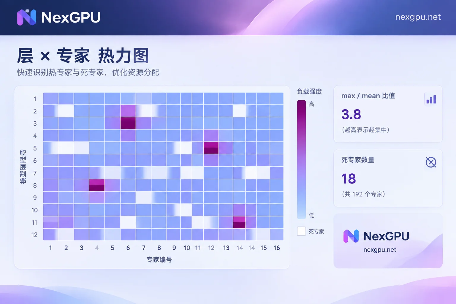
Step 2: Confirm the balancing loss is actually working
The auxiliary balancing loss is the primary means to suppress routing bias. Its curve should exist, be non-zero, and respond when skew increases. If the curve looks normal but skew still worsens, the loss weight may be too low to counteract the bias.
Common pitfalls during fine-tuning:
- Loss not added at all: In the Mixtral implementation in Transformers, the auxiliary loss is only added to the total loss via
router_aux_loss_coefwhenoutput_router_logitsis enabled. Many fine-tuning scripts do not enable this option by default. Implementations may vary across versions; refer to the source code of your version. - Router is frozen: When fine-tuning with LoRA, if the target modules do not include the gating layer, the router weights will not update at all, and the auxiliary loss cannot take effect. The imbalance you see in this case comes from the combination of your data and the original routing.
- Using an auxiliary-loss-free approach: Strategies like DeepSeek-V3's auxiliary-loss-free method do not rely on a loss term for balancing but dynamically adjust a bias for each expert based on load, without gradients. Its effect is not visible on the loss curve; directly confirm that bias updates are enabled and monitor changes in expert bias values.
Step 3: Check if router logits are diverging numerically
If the logits output by the gating layer grow larger and larger, softmax becomes very sharp, and routing approaches "each token only recognizes one expert." It is advisable to additionally log:
- The maximum absolute value of router logits per layer;
- Router Z-Loss, i.e., the mean of squared logsumexp of logits.
If these two metrics rise in sync with load skew, the problem is more likely in the numerical stability of the gating layer. You can add z-loss or normalize the gating logits and observe whether skew is alleviated.
Step 4: Check the statistical scope of balancing loss and capacity settings
- Statistical scope: Early implementations like Megatron-Core may compute balancing loss only within a single GPU or local batch. If each batch comes from the same domain, forcing balance within the batch can actually suppress natural expert differentiation. The Qwen team's approach is to compute balance over the global batch. In this case, do not blindly increase the loss weight; first confirm the statistical scope.
- Capacity and dropping: When a capacity factor is set, the token drop rate should be monitored separately. A high drop rate means some tokens skip expert computation entirely, affecting performance. You can increase the capacity factor (at the cost of more memory) or switch to dropless MoE based on block-sparse operators like MegaBlocks.
Multi-GPU Inference (EP): First Find the Straggler GPU
Use a Profiler to distinguish "slow compute" from "slow communication"
When deploying EP on vLLM or SGLang, capture per-rank expert computation kernel time and dispatch/combine (i.e., All-to-All) wait times per GPU.
- One GPU's expert computation is significantly longer, and other GPUs' All-to-All waits increase accordingly: This is a classic load imbalance bucket effect.
- All GPUs have similar computation times, but communication is generally slow: The problem is more likely in inter-GPU interconnect or parallelism configuration, not expert popularity. Refer to How to Choose Between Tensor Parallelism and Pipeline Parallelism and re-evaluate the parallelism strategy.
Use real traffic to count expert hits
When stress-testing with random prompts, expert distribution often looks uniform but skew only appears in production. It is recommended to sample real requests and count hit counts per expert ID per layer, focusing on two types of traffic: vision tokens in multimodal requests and vertical domain instructions. They tend to concentrate on a few fixed experts. After identifying hot expert IDs, check which GPU they are placed on. If several hot experts happen to be adjacent and assigned to the same rank, that GPU becomes the bottleneck.
Solution: Remap or replicate hot experts
vLLM provides an Expert Parallel Load Balancer (EPLB) that can rearrange expert placement across GPUs based on runtime load statistics, and can also replicate hot experts redundantly across multiple GPUs for load sharing. Two caveats: redundant replicas consume extra memory, and rearrangement itself has overhead. Parameter names vary across versions; refer to the vLLM documentation for your version before enabling.
What to Pay Attention to When Debugging on Rented GPUs
- Decide how many GPUs to rent based on the problem type: Routing statistics on the training side (steps 1 to 3 above) can be done with a single GPU running a small-batch forward pass, so you don't need to rent multiple GPUs initially. Tail latency issues in EP inference must be reproduced on a real multi-GPU node, and the inter-GPU interconnect directly affects All-to-All time, so consider interconnect when selecting nodes.
- Use ready-made images for the environment: On NexGPU, you can deploy vLLM or PyTorch images with one click from image templates, saving time on environment setup and starting Profiler and statistics scripts directly.
- Save results before destroying: Write Profiler traces and per-layer routing statistics to persistent storage. After shutdown, compute fees stop but storage fees continue; after instance destruction, all fees stop and data is deleted. So download results before destruction.
If the problem can only be reproduced under multi-node EP and you need to evaluate multi-node or cluster resources, you can contact NexGPU sales to discuss multi-GPU solutions.