 NexGPU-算力租赁,GPU服务器,GPU云算力,AI服务器租用-新闻博客
First, clarify where the compute cost of the Prefill phase and the bandwidth cost of the Decode phase each dominate, then determine the hardware specifications accordingly.
The Cost Structure of Inference GPUs: What Compute, Memory Bandwidth, and Resident Memory Each Buy You
The value of an LLM inference GPU is not solely defined by peak compute power but by three separately accountable costs: the compute consumed in parallel processing input prompts, the memory bandwidth consumed by repeatedly moving weights and KV Cache during token-by-token generation, and the resident memory required for model weights and runtime overhead. During the Prefill phase, the model processes all input tokens in parallel, with arithmetic intensity as high as 200-400 ops/byte, making this load typically compute-bound. However, entering the Decode phase, each autoregressive generation step must fully read the model weights and KV Cache, causing arithmetic intensity to drop sharply to 60-80 ops/byte, shifting the load to memory-bandwidth-bound. This means the same GPU offers completely different cost-effectiveness in the two phases. If your workload features long inputs and short outputs, you are mainly paying for compute; if it features short inputs and long outputs, you are mainly paying for bandwidth.
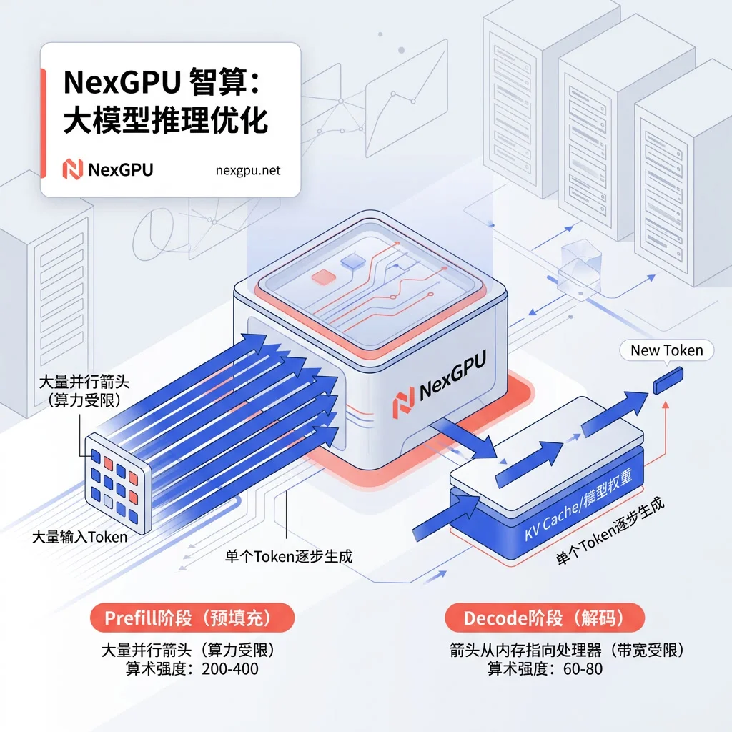
Why Decoding Latency Is Determined by Bandwidth: Most Compute Cores Are Waiting for Memory Data
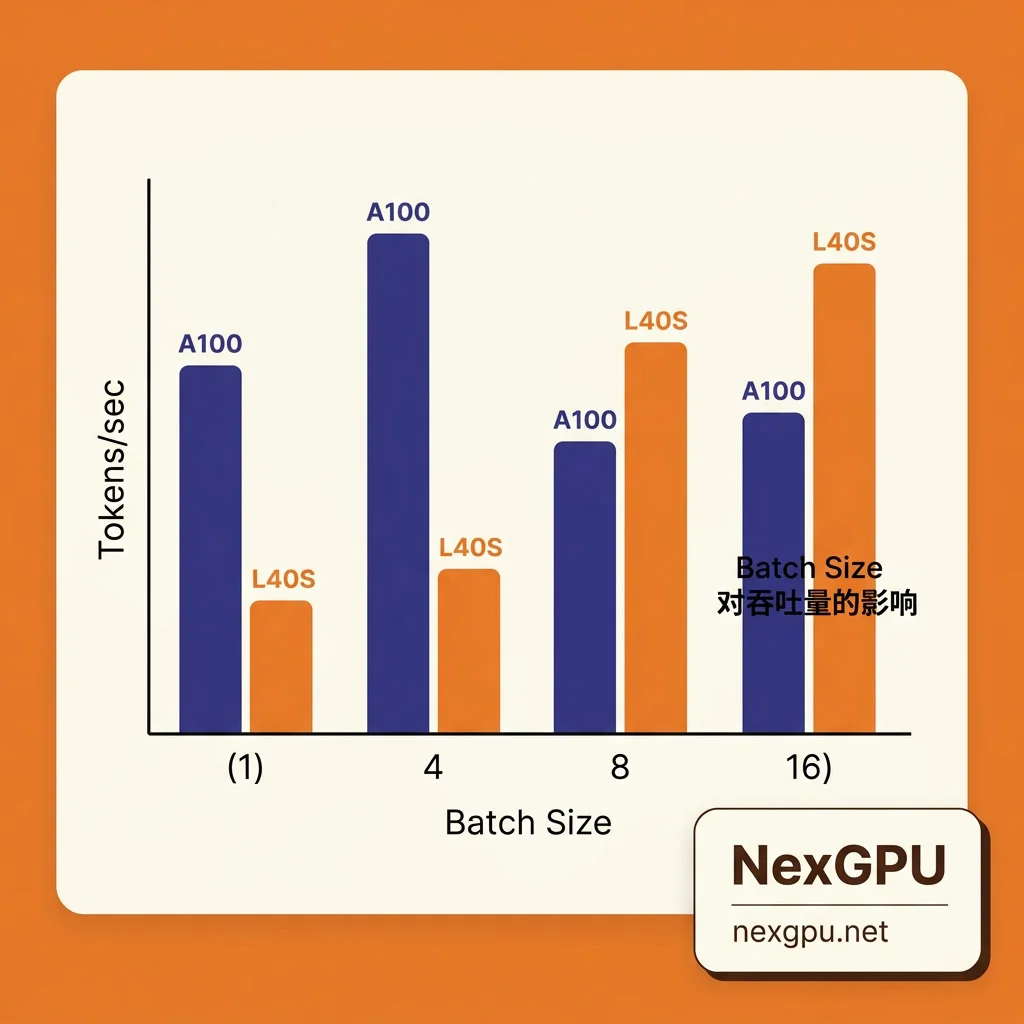
Many teams facing the question of "Is slow inference due to insufficient compute or insufficient memory bandwidth?" tend to stack more compute cards, but this is often a misjudgment. Token generation latency (ITL) is directly determined by memory bandwidth, because the core task in the Decode phase is reading data from memory, not performing complex calculations. Take the L40S and A100 80GB as examples. The former uses GDDR6 memory with 864 GB/s bandwidth, while the latter uses HBM2e memory with 2,039 GB/s bandwidth. The L40S's bandwidth is only about 42% that of the A100. In low-concurrency scenarios with Batch 1-4 or long-context single-stream scenarios, since the bottleneck is entirely on data movement, the A100 leverages its bandwidth advantage to deliver nearly 1.9 times higher decoding throughput. At this point, even if the L40S has higher theoretical FP8 compute, it cannot compensate for the waiting time caused by the bandwidth shortfall.
How to Reverse-Calculate the Memory Lower Bound: Weights, KV Cache, and Runtime Overhead Separately
When determining the memory capacity for an LLM inference GPU, you cannot only look at the model parameter size. You need to budget additively: model weights at the actual precision size, KV Cache that grows multiplicatively with concurrency and context length, and a fixed resident overhead for the inference engine and intermediate tensors. For MoE architecture models, it is strictly forbidden to estimate memory based on activated parameters, as all expert weights must be fully resident for dynamic routing. For example, a 671B-level model in FP8 precision still has a physical memory threshold above 700GB, far exceeding single-card capability. For common 48GB memory cards, they are typically only suitable for small models that have been deeply quantized or as part of a multi-card cluster; they cannot independently run large dense models. To assess the memory requirements of a specific model, refer to the detailed algorithm logic in The Impact of FP8 and INT4 Quantization on GPU Memory, and derive precise values based on your business's context length.
L40S vs A100 80GB: Low-Concurrency Single-Stream vs High-Concurrency Batch Processing
When selecting hardware, it is necessary to distinguish applicable scenarios based on concurrency depth. The table below shows key parameters and suitable ranges for the two mainstream card types:
| Parameter | NVIDIA L40S | NVIDIA A100 80GB |
|---|---|---|
| Memory Capacity | 48GB GDDR6 | 80GB HBM2e |
| Memory Bandwidth | 864 GB/s | 2,039 GB/s |
| Key Compute Metric | Native FP8: 733 TFLOPS | BF16: 312 TFLOPS |
| Best Fit Scenario | High-concurrency batch processing (Batch 8+) | Low concurrency (Batch 1-4) / long-context single-stream |
| Relative Bandwidth | Approx. 42% (vs A100) | Baseline 100% |
In high-concurrency scenarios with Batch 8+, the L40S leverages its native FP8 Tensor Core compute from the Ada Lovelace architecture to surpass the A100's BF16 compute in throughput. However, in low-concurrency or latency-sensitive long-text generation, its bandwidth disadvantage is apparent. Before long-term commitment to a card type, you can use NexGPU's multiple card types and pay-as-you-go capability to run the same workload on both a 48GB mid-range card and an 80GB HBM card, using real-world measurements instead of parameter tables to make decisions, avoiding mistakes based on peak specifications.
Precision Levels and Hardware Generations: What Tensor Cores FP16, FP8, and FP4 Require
Quantization benefits require hardware instruction support, and different generations of LLM inference GPUs support vastly different precision levels. The A100, based on the Ampere architecture, has third-generation Tensor Cores and lacks native FP4 hardware support; software emulation does not increase throughput. Therefore, the answer to "Can FP4 quantization accelerate on A100?" is no. The L40S, based on the Ada Lovelace architecture, has native FP8 support, effectively reducing memory usage and improving compute utilization. The Blackwell B200, with its fifth-generation Tensor Core, natively supports FP4 and offers 9,000 TFLOPS of dense compute. Readers need to confirm whether their current card can benefit from a specific precision; quantization plans should be determined based on hardware generation before selecting a card, rather than forcibly migrating afterward.
Migrating from a Multi-Card Cluster to B200-Class Nodes: What Workloads Are Worth Waiting For, and What Is Sufficient Now
The Blackwell B200 features 192GB HBM3e memory and 8TB/s bandwidth, allowing trillion-parameter or 671B-level MoE models to be shrunk into fewer nodes, significantly reducing cross-node tensor parallel communication overhead. For ultra-large model dense inference workloads constrained by cross-node communication, planning a migration to B200-class nodes is valuable. However, for high-concurrency services of medium and small models, existing card types such as A100 or L40S are already sufficient; there is no need to blindly wait for new architectures. On the supply side, B200 is mostly delivered in the form of invitation testing and commercial customization, with prices still dynamically adjusting. Before making a decision, first establish the same workload and context length as a baseline, and evaluate the communication bottleneck proportion of the current cluster.
Converting Rental Costs into Cost per Million Tokens: An Adjusted Calculation Based on Real Utilization
Final selection must return to cost accounting. The comprehensive cost per million tokens formula is: Cost per 1M tokens = (GPU hourly rental ÷ (actual TPS × 3,600)) × 1,000,000. In real business, due to request tidal effects, GPU average utilization typically ranges from 30% to 60%. If continuous batching (Continuous Batching) is not enabled to boost effective throughput, actual token costs can be 2 to 3 times higher than estimates based on peak load. Assuming a variable rental price, readers need to plug their own quotes into the formula for self-calculation. For example, if a card's hourly rental is $R$, and the actual TPS at Batch Size=1 is $T_1$, then unit cost directly depends on $T_1$, not the theoretical maximum. As seen in the case of DeepSeek-R1 Private Deployment GPU Configuration, TPS changes with different concurrency depths dramatically alter unit costs; never budget solely based on nominal compute.
FAQ
How to quickly determine whether the inference bottleneck is compute or bandwidth?
Look at the time ratio between Prefill and Decode phases. If the input is extremely long and time-to-first-token is high, it is mostly compute-bound; if the output is lengthy and every subsequent token generates slowly, even if GPU utilization seems low, it is usually memory-bandwidth-bound. You can verify by monitoring memory bandwidth utilization; if it is near saturation, it is a bandwidth bottleneck.
What model size can a 48GB GPU run?
It depends on quantization precision. In FP16, 48GB can only hold weights for a model of about 24B parameters. Adding KV Cache and runtime overhead, the actual dense model size that can run is smaller. With INT4 or FP8 quantization, larger parameter models can theoretically fit, but note that MoE models require all expert weights to be resident, making it difficult for a single 48GB card to run large MoE models.
Can older architecture cards achieve the same throughput gains from low-bit quantization as new architecture cards?
No. Cards with Ampere architecture like A100 lack native FP4 support. Software emulation not only fails to increase throughput but can also reduce efficiency due to conversion overhead. Only new architectures like Blackwell, which natively support FP4, can obtain significant compute density improvements from low-bit quantization.
How to convert rental costs for inference GPUs without losing money?
The key is to introduce an "actual utilization" correction factor. Do not use peak TPS directly; estimate TPS based on average concurrency from historical traffic. Also, be sure to enable continuous batching to improve resource reuse during idle times; otherwise, under tidal traffic, idle costs can inflate the unit token price by 2-3 times.
For low-concurrency low-latency scenarios versus high-concurrency throughput scenarios, which type of card should be preferred?
For low-concurrency scenarios sensitive to time-to-first-token and inter-token latency, cards with high HBM bandwidth (such as A100/H100) should be prioritized to reduce data waiting time. For high-concurrency batch processing scenarios seeking maximum overall throughput, cards with strong native FP8/FP16 compute and sufficient memory capacity (such as L40S) can be chosen to amortize the per-calculation cost.


Comments(0)